from topic_banner import new_topic
Classification with Linear Logistic Regression
Topics:
- Motivation and Setup
- Derivation
- Data Likelihood
- Maximizing the Data Likelihood
- Gradient Ascent Derivation
- Derivation Summary
- Implementation in Python
- Application to Parkinsons Data and Comparison to LDA and QDA
Motivation and Setup
new_topic('Motivation and Setup')
Recall that a linear model used for classification can result in masking. We discussed fixing this by using different shaped membership functions, other than linear.
Our first approach to this was to use generative models (Normal distributions) to model the data from each class, forming $p(\xv|C=k)$. Using Bayes' Theorem, we converted this to $p(C=k|\xv)$ and derived QDA and LDA.
Now we will derive a linear model that directly predicts $p(C=k|\xv)$, resulting in the algorithm called logisitic regression. It is derived to maximize the likelihood of the data, given a bunch of samples and their class labels.
Remember this picture?
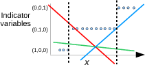
The problem was that the green line for Class 2 was too low. In fact, all lines are too low in the middle of x range. Maybe we can reduce the masking effect by
- requiring the function values to be between 0 and 1, and
- requiring them to sum to 1 for every value of x.
We can satisfy those two requirements by directly representing $p(C=k|\xv)$ as
$$ \begin{align*} p(C=k|\xv) = \frac{f(\xv;\wv_k)}{\sum_{m=1}^K f(\xv;\wv_m)} \end{align*} $$with $f(\xv;\wv) \ge 0$. We haven't discussed the form of $f$ yet, but $\wv$ represents the parameters of $f$ that we will tune to fit the training data (later).
This is certainly an expression that is between 0 and 1 for any $\xv$. And we have $p(C=k|\xv)$ expressed directly, as opposed to the previous generative approach of first modeling $p(\xv|C=k)$ and using Bayes' theorem to get $p(C=k|\xv)$.
Let's give the above expression another name
$$ \begin{align*} g_k(\xv) = p(C=k|\xv) = \frac{f(\xv;\wv_k)}{\sum_{m=1}^K f(\xv;\wv_m)} \end{align*} $$Derivation
new_topic('Derivation')
Whatever we choose for $f$, we must make a plan for optimizing its parameters $\wv$. How?
Let's maximize the likelihood of the data. So, what is the likelihood of training data consisting of samples $\{\xv_1, \xv_2, \ldots, \xv_N\}$ and class indicator variables
$$ \begin{align*} \begin{pmatrix} t_{1,1} & t_{1,2} & \ldots & t_{1,K}\\ t_{2,1} & t_{2,2} & \ldots & t_{2,K}\\ \vdots\\ t_{N,1} & t_{N,2} & \ldots & t_{N,K} \end{pmatrix} \end{align*} $$with every value $t_{n,k}$ being 0 or 1, and each row of this matrix contains a single 1? (We can also express $\{\xv_1, \xv_2, \ldots, \xv_N\}$ as an $N \times D$ matrix, but we will be using single samples $\xv_n$ more often in the following.)
Data Likelihood
new_topic('Data Likelihood')
The likelihood is just the product of all $p(C=\text{class of } n^\text{th}\text{ sample}\,|\,\xv_n)$ values for sample $n$. A common way to express this product, using those handy indicator variables is
$$ \begin{align*} L(\betav) = \prod_{n=1}^N \prod_{k=1}^K p(C=k\,|\, \xv_n)^{t_{n,k}} \end{align*} $$Say we have three classes ($K=3$) and training sample $n$ is from Class 2, then the product is
$$ \begin{align*} p(C=1\,|\,\xv_n)^{t_{n,1}} p(C=2\,|\,\xv_n)^{t_{n,2}} p(C=3\,|\,\xv_n)^{t_{n,3}} & = p(C=1\,|\,\xv_n)^0 p(C=2\,|\,\xv_n)^1 p(C=3\,|\,\xv_n)^0 \\ & = 1\; p(C=2\,|\,\xv_n)^1 \; 1 \\ & = p(C=2\,|\,\xv_n) \end{align*} $$This shows how the indicator variables as exponents select the correct terms to be included in the product.
Maximizing the Data Likelihood
new_topic('Maximizing the Data Likelihood')
So, we want to find $\wv$ that maximizes the data likelihood. How shall we proceed?
$$ \begin{align*} L(\wv) & = \prod_{n=1}^N \prod_{k=1}^K p(C=k\,|\, \xv_n) ^ {t_{n,k}} \end{align*} $$Right. Find the derivative with respect to each component of $\wv$, or the gradient with respect to $\wv$. But there is a mess of products in this. So...
Right again. Work with the natural logarithm $\log L(\wv)$ which we will call $LL(\wv)$.
$$ \begin{align*} LL(\wv) = \log L(\wv) = \sum_{n=1}^N \sum_{k=1}^K t_{n,k} \log p(C=k\,|\,\xv_n) \end{align*} $$Gradient Ascent
new_topic('Gradient Ascent')
For the faint-hearted, mathematically, scroll down and take a look at the mathematical expression just before "Derivation Summary". That is where we will end up!
Unfortunately, the gradient of $LL(\wv)$ with respect to $\wv$ is not linear in $\wv$, so we cannot simply set the result equal to zero and solve for $\wv$.
Instead, we do gradient ascent. (Why "ascent"?)
- Initialize $\wv$ to some value.
- Make small change to $\wv$ in the direction of the gradient of $LL(\wv)$ with respect to $\wv$ (or $\grad_{\wv} LL(\wv)$)
- Repeat above step until $LL(\wv)$ seems to be at a maximum.
where $\alpha$ is a constant that affects the step size.
Remember that $\wv$ is a matrix of parameters, with, let's say, columns corresponding to the values required for each $f$, of which there are $K-1$.
We can work on the update formula and $\grad_{\wv} LL(\wv)$ one column at a time
$$ \begin{align*} \wv_k \leftarrow \wv_k + \alpha \grad_{\wv_k} LL(\wv) \end{align*} $$and combine them at the end.
$$ \begin{align*} \wv \leftarrow \wv + \alpha (\grad_{\wv_1} LL(\wv), \grad_{\wv_2} LL(\wv), \ldots, \grad_{\wv_{K-1}} LL(\wv)) \end{align*} $$Remembering that $\frac{\partial \log h(x)}{\partial x} = \frac{1}{h(x)}\frac{\partial h(x)}{x}$ and that $p(C=k|\xv_n) = g_k(\xv_n)$
$$ \begin{align*} LL(\wv) & = \sum_{n=1}^N \sum_{k=1}^K t_{n,k} \log p(C=k\,|\,\xv_n)\\ & = \sum_{n=1}^N \sum_{k=1}^K t_{n,k} \log g_k(\xv_n)\\ \grad_{\wv_j} LL(\wv) & = \sum_{n=1}^N \sum_{k=1}^K \frac{t_{n,k}}{g_k(\xv_n)} \grad_{\wv_j} g_k(\xv_n) \end{align*} $$We also want $g_k(\xv_n)$ to be the probability $P(C=k | \xv_n)$, so need it to be between 0 and 1 for all $k$ and we want $\sum_{k=1}^K g_k(\xv_n) = 1$. And, hey, wouldn't it be super nice if $\grad_{\wv_j} g_k(\xv_n)$ includes the factor $g_k(\xv_n)$ so that it would cancel with the $g_k(\xv_n)$ in the denominator.
The following definition does all of this. This is often referred to as a softmax function.
$$ \begin{align*} g_k(\xv_n) & = \frac{\ebx{k}}{\sum_{m=1}^{K} \ebx{m}} \end{align*} $$Now we can work on $\grad_{\wv_j} g_k(\xv_n)$.
$$ \begin{align*} g_k(\xv_n) = \frac{\ebx{k}}{\sum_{m=1}^{K} \ebx{m}} \end{align*} $$So
$$ \begin{align*} \grad_{\wv_j} g_k(\xv_n) & = \grad_{\wv_j} \left (\frac{\ebx{k}}{\sum_{m=1}^{K} \ebx{m}} \right )\\ & = \grad_{\wv_j} \left [ \left (\sum_{m=1}^{K} \ebx{m} \right )^{-1} \ebx{k} \right ] \end{align*} $$Since $$ \begin{align*} \grad_{\wv_j} \ebx{k} &= \begin{cases} \xv_n \ebx{k}, & \text{if } k=j\\ 0 & \text{otherwise} \end{cases} \end{align*} $$ and $$ \begin{align*} \grad_{\wv_j} \sum_{m=1}^K-1 \ebx{m} &= \xv_n \ebx{k} \end{align*} $$ then $$ \begin{align*} \grad_{\wv_j} g_k(\xv_n) & = \grad_{\wv_j} \left (\frac{\ebx{k}}{\sum_{m=1}^{K} \ebx{m}} \right )\\ & = -1 \left (\sum_{m=1}^{K} \ebx{m} \right )^{-2} \xv_n \ebx{j} \ebx{k} + \left (\sum_{m=1}^{K} \ebx{m} \right )^{-1} \begin{cases} \xv_n \ebx{k},& \text{if} j=k\\ 0,& \text{otherwise} \end{cases}\\ & = -\frac{\ebx{k}}{\sum_{m=1}^{K} \ebx{m}} \frac{\ebx{j}}{\sum_{m=1}^{K} \ebx{j}} \xv_n + \begin{cases} \frac{\ebx{j}}{\sum_{m=1}^{K} \ebx{j}} \xv_n,& \text{if} j=k\\ 0,& \text{otherwise} \end{cases}\\ %& = \frac{\ebx{k}}{\sum_{m=1}^{K} \ebx{m} } & = - g_k(\xv_n) g_j(\xv_n) \xv_n + \begin{cases} g_j(\xv_n) \xv_n,^ \text{if} j=k\\ 0,& \text{otherwise} \end{cases}\\ & = g_k(\xv_n) (\delta_{jk} - g_j(\xv_n)) \xv_n \end{align*} $$ where $\delta_{jk} = 1$ if $j=k$, 0 otherwise.
Substituting this back into the log likelihood expression, we get
$$ \begin{align*} \grad_{\wv_j} LL(\wv) & = \sum_{n=1}^N \sum_{k=1}^K \frac{t_{n,k}}{g_k(\xv_n)} \grad_{\wv_j} g_k(\xv_n)\\ & = \sum_{n=1}^N \sum_{k=1}^K \frac{t_{n,k}}{g_k(\xv_n)} \left (g_k(\xv_n) (\delta_{jk} - g_j(\xv_n)) \xv_n \right )\\ & = \sum_{n=1}^N \left ( \sum_{k=1}^K t_{n,k} \delta_{jk} - g_j(\xv_n) \sum_{k=1}^K t_{n,k} \right ) \xv_n\\ & = \sum_{n=1}^N (t_{n,j} - g_j(\xv_n)) \xv_n \end{align*} $$which results in this update rule for $\wv_j$
$$ \begin{align*} \wv_j \leftarrow \wv_j + \alpha \sum_{n=1}^N (t_{n,j} - g_j(\xv_n)) \xv_n \end{align*} $$How do we do this in python? First, a summary of the derivation.
Derivation Summary
new_topic('Derivation Summary')
$P(C=k\,|\,\xv_n)$ and the data likelihood we want to maximize:
$$ \begin{align*} g_k(\xv_n) & = P(C=k\,|\,\xv_n) = \frac{f(\xv_n;\wv_k)}{\sum_{m=1}^{K} f(\xv_n;\wv_m)}\\ f(\xv_n;\wv_k) & = \left \{ \begin{array}{ll} \ebx{k}; & k < K\\ 1;& k = K \end{array} \right .\\ L(\wv) & = \prod_{n=1}^N \prod_{k=1}^K p(C=k\,|\, \xv_n) ^{t_{n,k}}\\ & = \prod_{n=1}^N \prod_{k=1}^K g_k(\xv_n)^{t_{n,k}} \end{align*} $$Gradient of log likelihood with respect to $\wv_j$:
$$ \begin{align*} \grad_{\wv_j} LL(\wv) & = \sum_{n=1}^N \sum_{k=1}^K \frac{t_{n,k}}{g_k(\xv_n)} \grad_{\wv_j} g_k(\xv_n)\\ %& = \sum_{n=1}^N \left ( \sum_{k=1}^K t_{n,k} \delta_{jk} - % g_j(\xv_n) \sum_{k=1}^K t_{n,k} \right )\\ & = \sum_{n=1}^N \xv_n (t_{n,j} - g_j(\xv_n)) \end{align*} $$which results in this update rule for $\wv_j$
$$ \begin{align*} \wv_j \leftarrow \wv_j + \alpha \sum_{n=1}^N (t_{n,j} - g_j(\xv_n)) \xv_n \end{align*} $$Implementation in Python
new_topic('Implementation in Python')
Update rule for $\wv_j$
$$ \begin{align*} \wv_j \leftarrow \wv_j + \alpha \sum_{n=1}^N (t_{n,j} - g_j(\xv_n)) \xv_n \end{align*} $$What are shapes of each piece? Remember that whenever we are dealing with weighted sums of inputs, as we are here, add the constant 1 to the front of each sample.
- $\xv_n$ is $(D+1) \times 1$ ($+1$ for the constant 1 input)
- $\wv_j$ is $(D+1) \times 1$
- $t_{n,j} - g_j(\xv_n)$ is a scalar
So, this all works. But, notice the sum is over $n$, and each term in the product as $n$ components, so we can do this as a dot product.
Let's remove the sum and replace subscript $n$ with *.
$$ \begin{align*} \wv_j &\leftarrow \wv_j + \alpha \sum_{n=1}^N (t_{n,j} - g_j(\xv_n)) \xv_n\\ \wv_j &\leftarrow \wv_j + \alpha (t_{*,j} - g_j(\xv_*)) \xv_*\\ \end{align*} $$What are shapes of each piece?
- $(t_{*,j} - g_j(\xv_*))$ is $N \times 1$
- $\xv_* = X$ is $N \times (D+1)$
- $\wv_j$ is $(D+1) \times 1$
So, this will work if we transpose $X$ and premultiply it and define $g$ as a function that accepts $\Xv$.
$$ \begin{align*} % \wv_j &\leftarrow \wv_j + \alpha (t_{*,j} - % g(\xv_*;\wv_j)) \xv_*\\ \wv_j &\leftarrow \wv_j + \alpha \Xv^T (t_{*,j} - g_j(\Xv)) \end{align*} $$Let's keep going...and try to make this expression work for all of the $\wv$'s. Playing with the subscripts again, replace $j$ with *.
$$ \begin{align*} \wv_j &\leftarrow \wv_j + \alpha \Xv^T (t_{*,j} - g_j(\Xv))\\ \wv_* &\leftarrow \wv_* + \alpha \Xv^T (t_{*,*} - g_*(\Xv)) \end{align*} $$Now what are shapes?
- $\wv_* = \wv$ is $(D+1) \times K$
- $t_{*,*} = T$ is $N \times K$
- $g_*(\Xv)$ is $N \times (K-1)$
- $t_{*,*} - g_*(\Xv)$ is $N \times K$
- So, $\Xv^T (t_{*,*} - g_*(\Xv))$ is $(D+1) \times K$
- So, $\Xv^T (T - g(\Xv))$ is $(D+1) \times K$
Now our update equation for all $\wv$'s is
$$ \begin{align*} \wv &\leftarrow \wv + \alpha \Xv^T (T - g(\Xv)) \end{align*} $$We had defined, for $k = 1,\ldots, K$,
$$ \begin{align*} g_k(\xv) &= \dfrac{\ebx{k}}{\sum_{m=1}^K \ebx{m}} \end{align*} $$Changing these to handle all samples $\Xv$ and all parameters $\wv$ we have
$$ \begin{align*} g(\Xv) & = \frac{e^{\Xv \wv}}{\text{rowSums}(e^{\Xv \wv})} \end{align*} $$Given training data $\Xv$ ($N\times (D+1)$) and class indicator variables $T$ ($N \times K)$), these expressions can be performed with the following code.
First, we need a function to create indicator variables from the class labels, to get
$$ \begin{bmatrix} 1\\ 2\\ 2\\ 1\\ 3 \end{bmatrix} \Rightarrow \begin{bmatrix} 1 & 0 & 0\\ 0 & 1 & 0\\ 0 & 1 & 0\\ 1 & 0 & 0\\ 0 & 0 & 1 \end{bmatrix} $$%load_ext autoreload
%autoreload 2
import numpy as np
import matplotlib.pyplot as plt
def make_indicator_vars(T):
    # Make sure T is two-dimensional. Should be nSamples x 1.
    if T.ndim == 1:
        T = T.reshape((-1, 1))
    return (T == np.unique(T)).astype(int)
T = np.array([1,2,2,1,3]).reshape((-1,1))
T
make_indicator_vars(T)
def g(X, w):
    fs = np.exp(X @ w)  # N x K
    denom = np.sum(fs, axis=1).reshape((-1, 1))
    gs = fs / denom
    return gs
The function g is sometimes called the softmax function.
def softmax(X, w):
    fs = np.exp(X @ w)  # N x K
    denom = np.sum(fs, axis=1).reshape((-1, 1))
    gs = fs / denom
    return gs
Now the updates to $\wv$ can be formed with code like this.
TI = make_indicator_vars(T)
w = np.zeros((X.shape[1], TI.shape[1]))
alpha = 0.0001
for step in range(1000):
    Y = softmax(X, w)
    w = w + alpha * X.T @ (TI - Y)
Application to Parkinsons Data and Comparison with LDA and QDA
new_topic('Application to Parkinsons Data and Comparison with LDA and QDA')
Here is code for applying linear logistic regression to the Parkinsons data from last lecture: parkinsons data set
import pandas as pd
data = pd.read_csv('parkinsons.data')
data.shape
X = data
X = X.drop(['status', 'name'], axis=1)
Xnames = X.columns.tolist()
X = X.values

T = data['status'].values
T = T.reshape((-1, 1))
Tname = 'status'

X.shape, Xnames, T.shape, Tname
def standardize(X, mean, stds):
    return (X - mean) / stds
import qdalda # from previous lecture
To generate our training, validation and testing partitions we need to partition data into folds on a class by class basis to make each fold have appoximately the same proportion of samples from each class. Here is a function that does this. This form of partitioning is referred to as "stratified".
def generate_stratified_partitions(X, T, n_folds, validation=True, shuffle=True):
    '''Generates sets of  Xtrain,Ttrain,Xvalidate,Tvalidate,Xtest,Ttest
      or
       sets of Xtrain,Ttrain,Xtest,Ttest if validation is False
    Build dictionary keyed by class label. Each entry contains rowIndices and start and stop
    indices into rowIndices for each of n_folds folds'''

    def rows_in_fold(folds, k):
        all_rows = []
        for c, rows in folds.items():
            class_rows, starts, stops = rows
            all_rows += class_rows[starts[k]:stops[k]].tolist()
        return all_rows

    def rows_in_folds(folds, ks):
        all_rows = []
        for k in ks:
            all_rows += rows_in_fold(folds, k)
        return all_rows

    row_indices = np.arange(X.shape[0])
    if shuffle:
        np.random.shuffle(row_indices)
    folds = {}
    classes = np.unique(T)
    for c in classes:
        class_indices = row_indices[np.where(T[row_indices, :] == c)[0]]
        n_in_class = len(class_indices)
        n_each = int(n_in_class / n_folds)
        starts = np.arange(0, n_each * n_folds, n_each)
        stops = starts + n_each
        stops[-1] = n_in_class
        folds[c] = [class_indices, starts, stops]

    for test_fold in range(n_folds):
        if validation:
            for validate_fold in range(n_folds):
                if test_fold == validate_fold:
                    continue
                train_folds = np.setdiff1d(range(n_folds), [test_fold, validate_fold])
                rows = rows_in_fold(folds, test_fold)
                Xtest = X[rows, :]
                Ttest = T[rows, :]
                rows = rows_in_fold(folds, validate_fold)
                Xvalidate = X[rows, :]
                Tvalidate = T[rows, :]
                rows = rows_in_folds(folds, train_folds)
                Xtrain = X[rows, :]
                Ttrain = T[rows, :]
                yield Xtrain, Ttrain, Xvalidate, Tvalidate, Xtest, Ttest
        else:
            # No validation set
            train_folds = np.setdiff1d(range(n_folds), [test_fold])
            rows = rows_in_fold(folds, test_fold)
            Xtest = X[rows, :]
            Ttest = T[rows, :]
            rows = rows_in_folds(folds, train_folds)
            Xtrain = X[rows, :]
            Ttrain = T[rows, :]
            yield Xtrain, Ttrain, Xtest, Ttest
for Xtrain, Ttrain, Xval, Tval, Xtest, Ttest in generate_stratified_partitions(X, T, 4):
    print(f'{len(Ttrain)} {np.mean(Ttrain == 0):.3f} {len(Tval)} {np.mean(Tval == 0):.3f} {len(Ttest)} {np.mean(Ttest == 0):.3f}')
print('\n', np.mean(T == 0))
Now we can write a function that can iterate over all ways of making training, validation and test sets from n_folds partitions and train QDA, LDA and linear logistic regression models to the data.
In the following function the break statement at the end of the for loop stops execution after just one run of the cross-validation method, to save time. To use all runs, we would have to calculate the mean errors, or accuracies, over all cross-validation runs.
def run_park_logreg(X, T, n_folds):

    for Xtrain, Ttrain, Xtest, Ttest in generate_stratified_partitions(X, T, n_folds, validation=False):

        means,stds = np.mean(Xtrain, 0), np.std(Xtrain ,0)
        Xtrains = standardize(Xtrain, means, stds)
        Xtests = standardize(Xtest, means, stds)

        Xtrains1 = np.hstack(( np.ones((Xtrains.shape[0], 1)), Xtrains))
        Xtests1 = np.hstack(( np.ones((Xtests.shape[0], 1)), Xtests))

        # New stuff for linear logistic regression

        TtrainI = make_indicator_vars(Ttrain)
        TtestI = make_indicator_vars(Ttest)

        w = np.zeros((Xtrains1.shape[1], TtrainI.shape[1]))
        likelihood = []
        alpha = 0.0001
        for step in range(10000):
            # forward pass
            gs = softmax(Xtrains1, w)
            # backward pass and weight update
            w = w + alpha * Xtrains1.T @ (TtrainI - gs)
            # convert log likelihood to likelihood
            likelihoodPerSample = np.exp( np.sum(TtrainI * np.log(gs)) / Xtrains.shape[0])
            likelihood.append(likelihoodPerSample)

        plt.figure(figsize=(8, 3))

        plt.subplot2grid((1, 4), (0, 0))
        plt.plot(likelihood)
        plt.ylabel('Likelihood')
        plt.xlabel('Epoch')

        logregOutput = g(Xtrains1, w)
        predictedTrain = np.argmax(logregOutput, axis=1)
        logregOutput = g(Xtests1, w)
        predictedTestLR = np.argmax(logregOutput, axis=1)

        print("LogReg: Percent correct: Train {:.3g} Test {:.3g}".format(percent_correct(predictedTrain, Ttrain),
                                                                         percent_correct(predictedTestLR, Ttest)))

        # Previous QDA, LDA code

        qda = qdalda.QDA()
        qda.train(Xtrain, Ttrain)
        qdaPredictedTrain = qda.use(Xtrain)
        qdaPredictedTest = qda.use(Xtest)
        print("   QDA: Percent correct: Train {:.3g} Test {:.3g}".format(percent_correct(qdaPredictedTrain, Ttrain),
                                                                         percent_correct(qdaPredictedTest, Ttest)))

        lda = qdalda.LDA()
        lda.train(Xtrain, Ttrain)
        ldaPredictedTrain = qda.use(Xtrain)
        ldaPredictedTest = qda.use(Xtest)
        print("   LDA: Percent correct: Train {:.3g} Test {:.3g}".format(percent_correct(ldaPredictedTrain, Ttrain),
                                                                         percent_correct(ldaPredictedTest, Ttest)))

        plt.subplot2grid((1, 4), (0, 1), colspan=3)
        plt.plot(Ttest, 'o-', label='Target')
        plt.plot(predictedTestLR, 'o-', label='LR')
        plt.plot(qdaPredictedTest, 'o-', label='QDA')
        plt.plot(ldaPredictedTest, 'o-', label='LDA')
        plt.legend()
        plt.ylabel('Class')
        plt.xlabel('Sample')
        plt.ylim(-0.1, 1.1)

        plt.tight_layout()

        break  # only do one data partition

def percent_correct(p, t):
    return np.sum(p.ravel()==t.ravel()) / float(len(t)) * 100
run_park_logreg(X, T, 5)
run_park_logreg(X, T, 5)
run_park_logreg(X, T, 5)